How do we make predictions for crypto price data? Here, we summarize the main steps involved. First, we fetch the data using the REST api from a major exchange. Typically, we can only fetch data for 24-72 hours prior at one time (the max allowed with fine granularity). We can get product candles using the following command sequence in Python, where we must specify start and end dates and granurality (data frequency) as parameters.
json.loads(connect('https://api.exchange.coinbase.com/products/'+ asset_name +'/candles', param = params).text)
Following this, we can build a data frame with columns ['utime','low','high','open','close','volume'] for each asset, where unix time format can be converted to custom format using the utcfromtimestamp function.

We calculate vwap data using this sample approximation with the average (low, high) price:

 
vwap = (avgp*volume).cumsum()/volume.cumsum();

Next, we must be able to merge data from nearby time queries. To do this, we match by date the latest data to the saved data, then append the previous data with the latest data from the first matching time point.

 
    inter_ind = times_latest[times_latest == times_saved_select].index[0]; 
    price_nvals = price_latest[inter_ind+1:].values;
    volume_nvals = volume_latest[inter_ind+1:].values;
    vwap_nvals = vwap_latest[inter_ind+1:].values;
    price_saved_new = np.concatenate([price_saved, price_nvals],axis=0)
    volume_saved_new = np.concatenate([volume_saved, volume_nvals],axis=0)
    vwap_saved_new = np.concatenate([vwap_saved, vwap_nvals],axis=0)

Finally, we load the combined data for modeling and prediction. We arrange a data frame with the combined time series data (for price, volume, and vwap) and apply a VAR (multivariate time series) model on the data for different orders.

 
    price_and_vol = pd.DataFrame(zip(df_price, df_volume, df_vwap), columns=["price", "volume", "vwap"]);
    model = VAR(price_and_vol);
    model_aics = [];
    for order in morders:
        model_fit = model.fit(order);
        model_aics.append(model_fit.aic);
    end

We can compare performance for different orders by obtaining the corresponding AIC values, looking for the smallest. Next, we can repeat the modeling with the log values of the differenced data vectors. In both cases, we obtain predictions from the VAR model:


model_fit = model.fit(morder);
pred = model_fit.forecast(...)

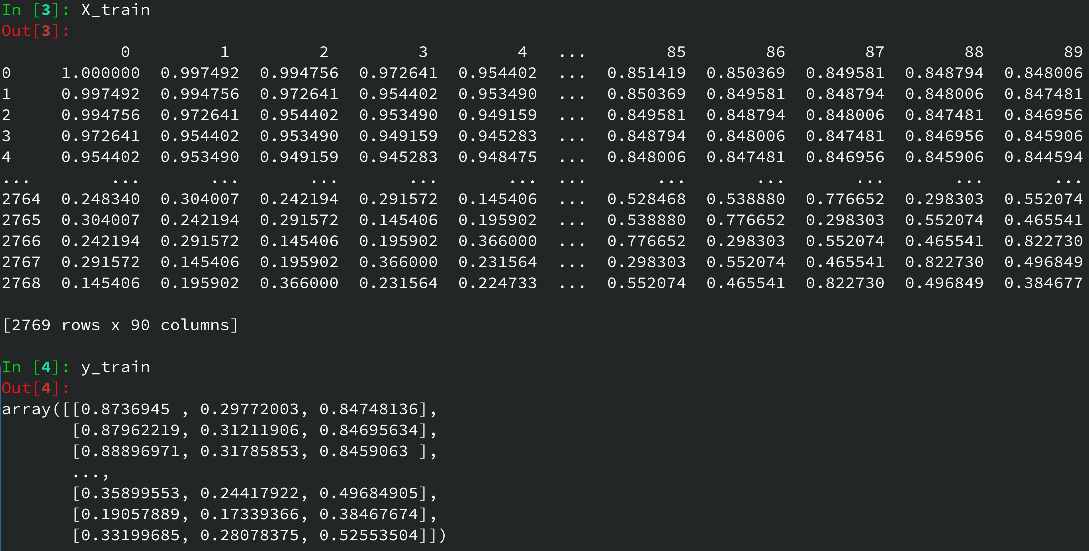
For machine learning, the data must be put into a tabular form, whereby each row has price, volume, and vwap data for times 1 to J-1, and the training y vector has the outputs for time J, where J increases to the last available data number.

The y vector (a matrix here), contains columns of predicted price, volume, and vvwap data for the next time value. Optionally, we can restrict this to only the price. This way, we can make a train using known data and a test set using the last few values for predicting the next, unknown set of values. We can then append this prediction to the data and retrain the model (with an additional data row), then predicting the next set of values.

For indicators, we compute the relative strength index, RSI = 100 - (100 / (1 + RS)), with RS the avg gain / avg_loss ratio over a set time period and the exponential moving average, EMA = (Close - Previous EMA) * 2 / (nperiods + 1) + Previous EMA for use with the moving average convergence divergence (MACD) indicator. The MACD line = 12-period EMA - 26-period EMA, the Signal line = 9-period EMA of the MACD line, and the difference between the MACD and Signal lines, known as the MACD histogram. Positive histogram bars indicate that the MACD line is above the signal line, suggesting bullish momentum. The outputs on the indicators can be used to judge potential to buy or sell signals. For example, if the MACD generates a buy signal, and the RSI is also above 50 and rising, it suggests stronger bullish momentum, and if the MACD generates a sell signal, and the RSI is below 50 and falling, it suggests stronger bearish momentum.

back to home